
-DSLOWREAD flag.
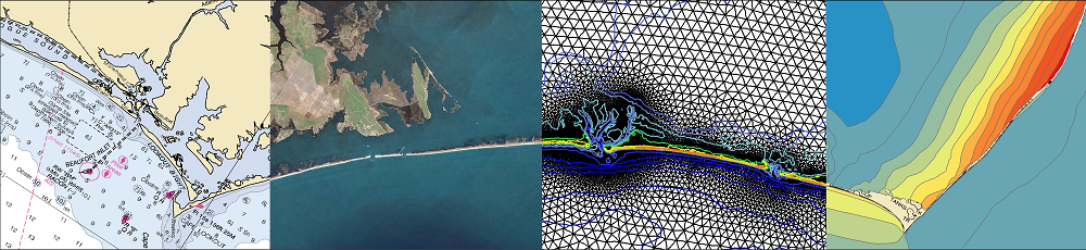
FigureGen is a Fortran program that creates images for ADCIRC files. It reads mesh files (fort.14, etc.), nodal attributes files (fort.13, etc.) and output files (fort.63, fort.64, maxele.63, etc.). It plots contours, contour lines, and vectors. Using FigureGen, you can go directly from the ADCIRC input and output files to a presentation-quality figure, for one or multiple time snaps.
This program started from a script written by Brian Blanton, and I converted it to Fortran because I am more familiar with that language. It now contains code written by John Atkinson, Zach Cobell, Howard Lander, Chris Szpilka, Matthieu Vitse, and others. But, at its core, FigureGen behaves like a script, and it uses system calls to tell other software how to generate the figure(s).
This example depicts hypothetical oil transport in the northern Gulf of Mexico. The oil spill is represented by Lagrangian particles and initialized with the observed conditions of 29 June 2010, but then the wind forcing of Hurricane Ike (2008) is applied. Oil is pushed into the marshes along the entire coastline of southern Louisiana.
UPDATED 2013/09/30: We published recently an application of FigureGen to the real-time visualization of storm surge forecasts during Hurricane Isaac (2012). This publication describes how FigureGen interfaces between the ADCIRC files and the Generic Mapping Tools (GMT) to produce raster images. If you find FigureGen to be useful in preparing figures for a presentation or publication, then we would appreciate a citation to this work, perhaps with a line in your acknowledgments:
“Some ADCIRC visualizations were produced with FigureGen (Dietrich et al., 2013).”
Note to Existing Users:
It is recommended that you upgrade to this new version, especially because it contains many bug fixes from the previous version, and thus it is much more robust.
It also contains several new features:
- Compatibility with the NetCDF-formatted output files from SWAN+ADCIRC. These files are much smaller than the standard ASCII-formatted output files, and FigureGen can process them more quickly. This new feature is described in Example 12.
- Capability to plot Lagrangian particles from the tracking code. This new feature was very useful in our oil spill modeling effort, as described below in Example 13.
- Capability to plot background images behind the rest of the plot. We added a representation of the observed oil spill from the satellite imagery, as described below in Examples 11 and 14. This feature can be used to add any geo-referenced image.
The source files are linked with notes on how to compile and run the code. Then several examples are provided, along with the necessary input files, to show how to exercise the many features of FigureGen.
System Requirements:
FigureGen relies on other software as it makes images from ADCIRC-related files. You will need to install these software packages on your system before using FigureGen.
- Generic Mapping Tools (GMT) is the software package that plots the contours, contour lines, etc. and produces a PostScript file containing the figure. The GMT software package is actually a suite of executable programs, of which FigureGen uses only a subset. Note that FigureGen v.49 only works with GMT 4.5 or higher! We use their
ps2rastercommand to convert the PostScript files to raster images, and theps2rastercommand was not implemented until GMT 4.5. - GhostScript is the software package that converts PostScript files into different formats, including the raster format used by FigureGen. GhostScript is typically installed on Unix systems, so it may already be available on your system.
- ImageMagick is a software package for the manipulation and conversion of images. This software is optional! It is only required when FigureGen adds background images to the plots, as shown in Examples 11 and 14 below. In that case, the
convertcommand needs to be available from ImageMagick. Otherwise, this software can be ignored.
Source Files:
The source code is FigureGen49.F90. This code will ask the user for and then read an input file containing information about which files to plot and how. FigureGen will plot the contours of both elevation-type (fort.63, maxele.63, maxwvel.63, etc.) and velocity-type (fort.64, fort.74, etc.) output files, mesh (fort.14) files, and nodal attributes (fort.13) files. You can specify a color palette to use by creating and saving a palette in SMS. You can convert units automatically. You can specify the lat/lon box to plot. And, perhaps most importantly, you can run FigureGen in parallel, so that you can create multiple images in a short amount of time. Example input files are provided at the bottom of this page.
Also, although many of the examples use different color palettes, it is best to start with the Default2.pal palette for most applications. This palette has been constructed painstakingly to contain the appropriate amount of purple. FigureGen will accept any color palette in SMS format, though, so you can feel free to experiment.
How to Compile:
As stated above, FigureGen is written so that the source file contains instructions for both serial and parallel implementations, and it has been extended for use with NetCDF. Serial compilation is fairly straight-forward; the following example uses the Portland Group compiler:
pgf90 FigureGen49.F90 -o FigureGen49.exe
To compile for use in a parallel computing environment, you should add the -DCMPI pre-compiler flag. The following example uses the Intel compilers and MVAPICH2:
mpif90 FigureGen49.F90 -DCMPI -o FigureGen49.exe
You can add the NetCDF functionality by using the -DNETCDF pre-compiler flag and including the necessary directories and libraries. The following example uses the Intel compilers and NetCDF version 4.1.1:
ifort FigureGen49.F90 -DNETCDF -I/opt/apps/intel11_1/netcdf/4.1.1/include

            -L/opt/apps/intel11_1/netcdf/4.1.1/lib -lnetcdf -o FigureGen49.exe
I have also used the GNU Fortran compiler without any problems. Please let me know if you have any questions about compiling FigureGen.
How to Run:
The serial version of FigureGen can be executed from the command prompt:
./FigureGen49.exe
And the parallel version can be executed typically with a command like:
mpirun -np 32 ./FigureGen49.exe
depending on the system, of course. In both cases, FigureGen will ask the user for the name of the input file, and then it will proceed with the generation of the figure(s).
There are other tricks for high-level users of FigureGen.
- Command-line arguments. This new version 49 of FigureGen will also accept command-line arguments for the name of the input file and/or the version number. For example, the command:
./FigureGen49.exe -I FG49_01_SL16v31_Bathy_SELA.inp -V 49would instruct FigureGen that the input file is named
FG49_01_SL16v31_Bathy_SELA.inpand that it is formatted for version 49. FigureGen will read from this input file without prompting the user for the file name. This new feature can be useful in parallel computing environments.For the version number, FigureGen will accept and process input files that are formatted for previous releases, including versions 41, 32, and 26. So FigureGen is backward-compatible! You can re-use input files with this new version 49.
- Loose coupling with ADCIRC. You can couple loosely FigureGen with an ADCIRC simulation and create images as the simulation is running. FigureGen will try to read data from your specified files (fort.63, fort.74, etc.), but it will not die if the data has not yet been written. Instead, it will output a message like:
Core 0003 is trying to read from the end of fort.63.Then it will wait a minute and try again. In this way, your ADCIRC simulation can be running and writing the files, FigureGen can be reading the files and generating images, and you will have a full set of images ready for you when your simulation is complete.
Note that, if you see that message and you’re not trying to run FigureGen concurrently with ADCIRC, then you know something is wrong with your FigureGen input file. Either you are trying to plot a time snap that doesn’t exist, or you’ve set something else incorrectly. Double-check that your existing ADCIRC files contain the time snaps that you’re trying to visualize.
Updated 2012/08/27: This feature must now be activated by using the
-DSLOWREADflag when the code is compiled. This flag will enable the deliberate reading of the ADCIRC files as they become available. This style of reading is very slow, so it is not enabled by default.
Examples:
The rest of this page contains examples to show some of the capabilities of FigureGen. Input files are provided as a guide for new users. Note that all of the features can be mixed and matched, so you do not have to use the examples exactly as they are provided. Please feel free to mix and match. Let me know if you have any questions.
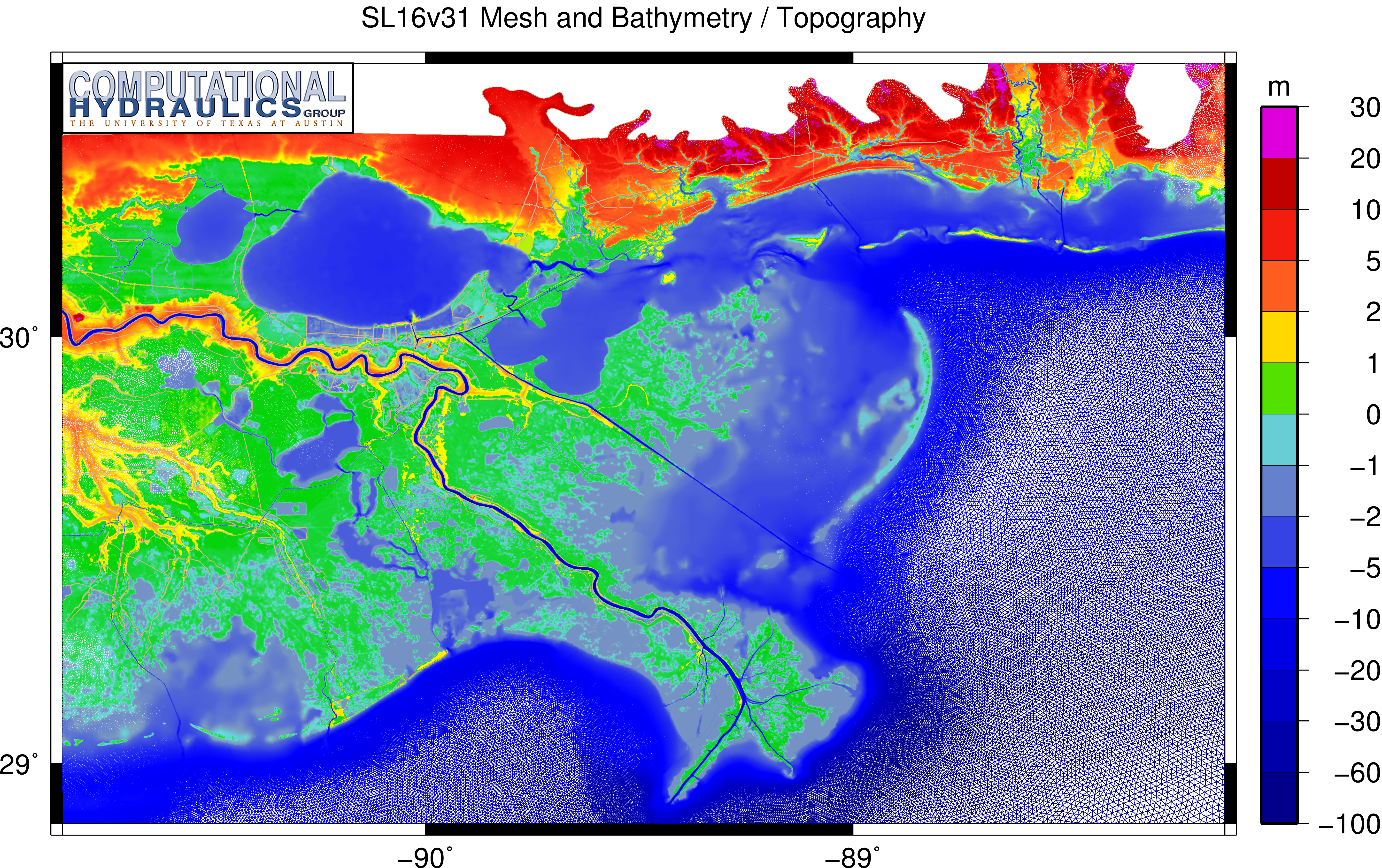
1. Bathymetry/topography with labels of landmarks.
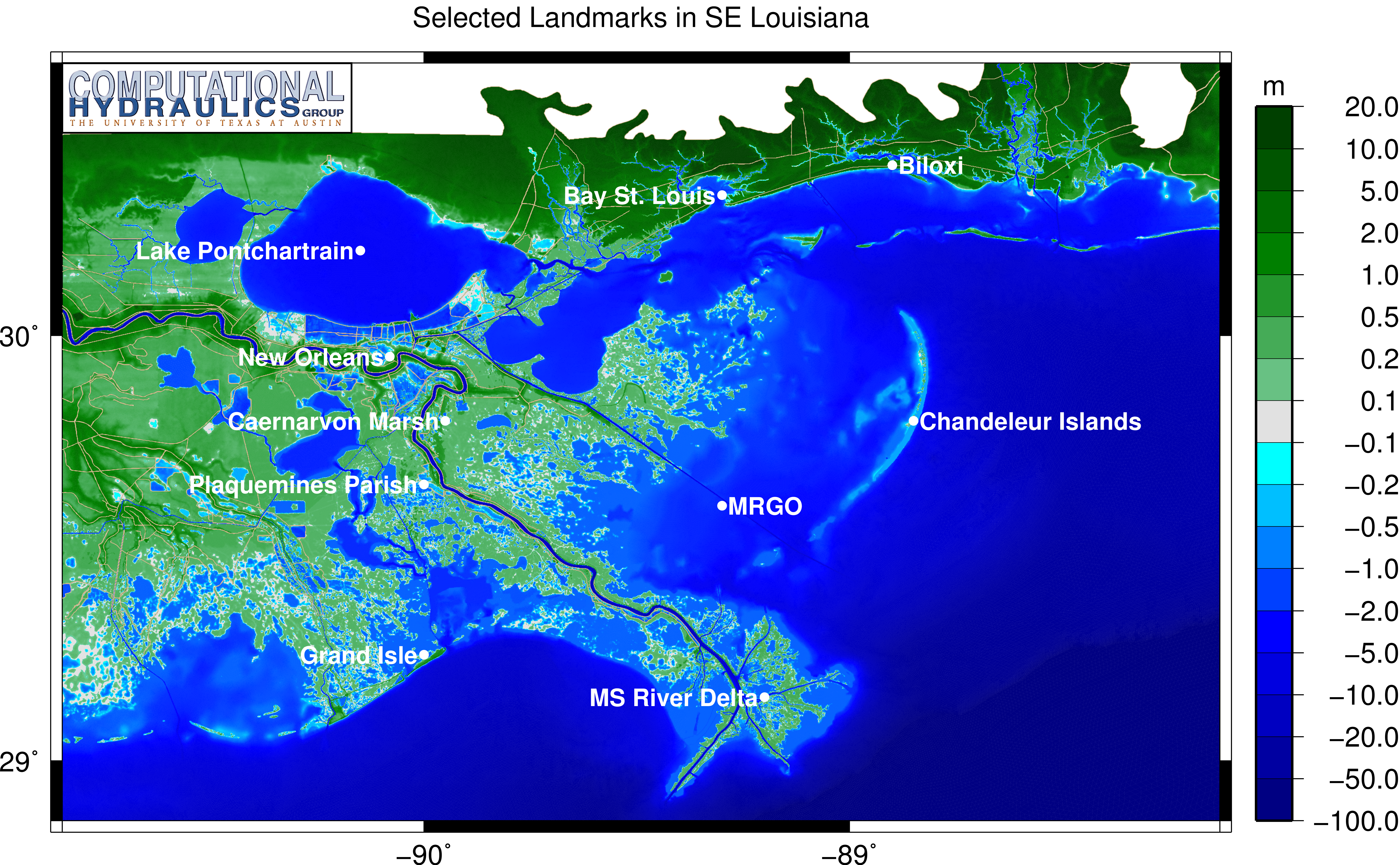
The image above shows the bathymetry and topography in our SL16 mesh, which has been validated for applications of hurricane waves and surge (here and here), as well as oil transport (here). This unstructured mesh offers unprecedented resolution in southeastern Louisiana. Note the intricate representation of the distributaries of the Mississippi River delta, the man-made channels such as the MRGO, and the marshes and bayou throughout the region.
- FG49_01_Files
- FG49_01_SL16v31_Bathy_SELA.inp
- TopoBlueGreen.pal
- TopoBlueGreen.txt
- Labels.txt
- CHG.eps
The bathymetry and topography are plotted with contours of blue and green, respectively, as specified in the SMS-friendly palette file. We also specify a text file with the desired contour intervals for the plot. The main portion of this text file contains two columns: the first column contains the contour intervals, while the second column indicates which intervals should have their colors replaced with white. In this example, we force values near zero to be plotted as white, to better indicate the location of the coastline. These contour intervals are also used in the example at the top of this page.
The labels are specified in an external file. The format of this file has been changed for the new version 49 of FigureGen, so that it now includes information about the font size and color. So each label is now specified with a line containing:
LabelText,Longitude,Latitude,Position,FontSize,FontColor
with no extra spaces. The position is any two-character specifier of the alignment in the horizontal (L,C,R) and vertical (T,M,B) directions. For example, to plot the marker to the right and bottom of the label, you would use the position specifier of RB. Most font colors are allowed; an extensive list is provided in the GMT Manual.
2. Mesh spacings with coastline schematic.
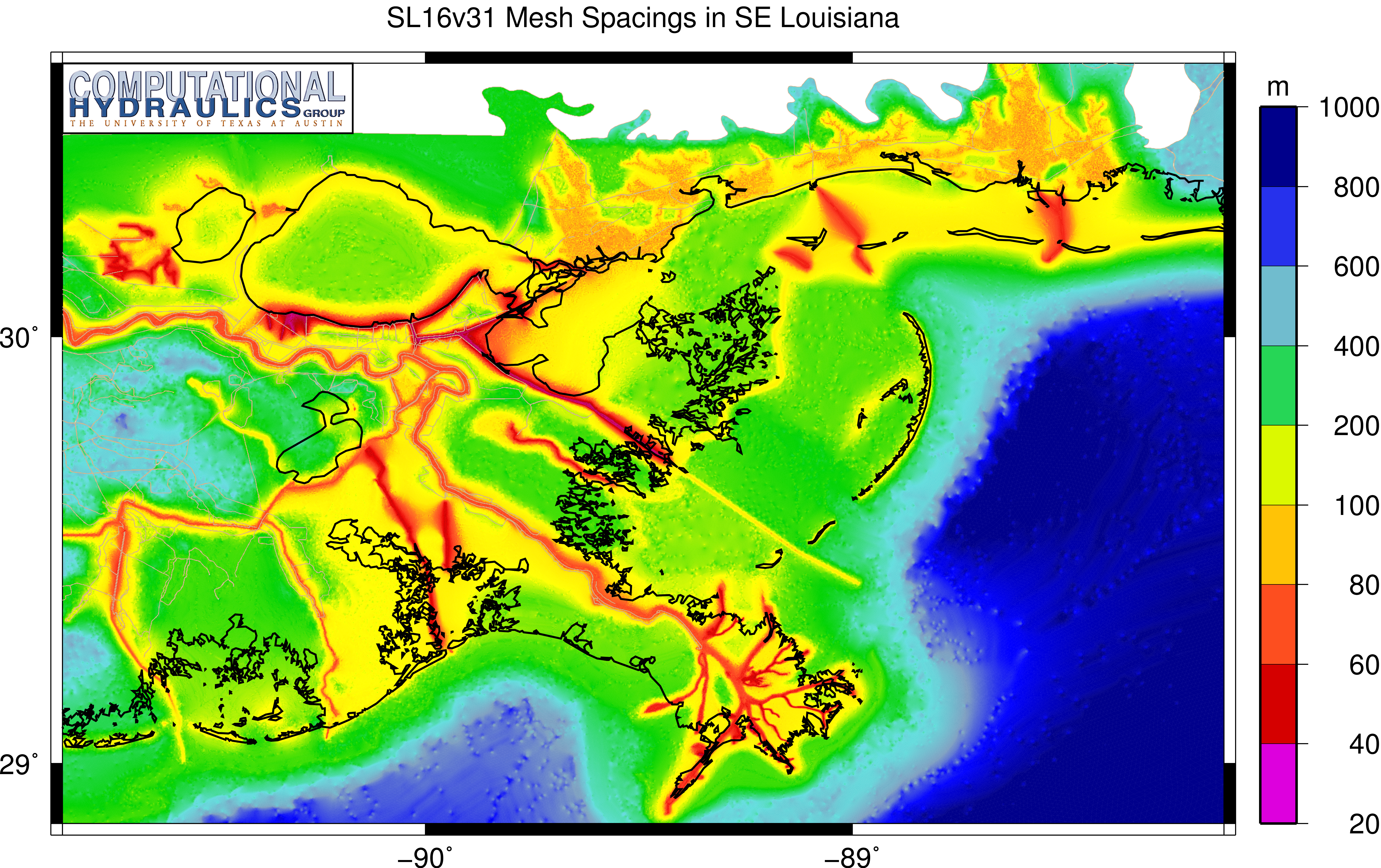
The high levels of resolution in the SL16 mesh are more obvious when the mesh spacings are contoured. The mesh spacings are about 1km on the continental shelf, 200m in the wave-breaking zones and inland, and 50m or less in the fine-scale channels and distributaries. The mesh spacings range downward to a minimum of about 20m.
- FG49_02_Files
- FG49_02_SL16v31_Grid-Size_SELA.inp
- GridSize.pal
- GridSize.txt
- CHG.eps
In figures like this example, in which the coastline is not well-defined, it is possible to add a schematic of the coastline using GMT. This feature is controlled by a line near the end of the FigureGen input file. The user can select the color of the schematic, as well as the complexity of the coastline and the inland water bodies. In this example, we have added a black coastline to better indicate how the resolution is increased beyond the barrier islands, behind the wave-breaking zones, and within the channels.
3. Mesh with coloring of bathymetry/topography.
Instead of contouring the bathymetry and topography, we can also plot it directly onto the unstructured mesh, as shown in this example. The SL16 mesh is so dense that most of the triangular elements cannot be seen at this scale. However, in the southeast corner of the image, it is possible to see the larger elements on the continental shelf. The elements are colored based on the bathymetry and topography at their adjacent vertices.
- FG49_03_Files
- FG49_03_SL16v31_Grid-Bath_SELA.inp
- FG49_03_SL16v31_Grid-Bath_SELA_GRF.inp
- FG49_03_SL16v31_Grid-Bath_SELA_KMZ.inp
- TopoRainbow.pal
- TopoRainbow.txt
- CHG.eps
- CHG.png
Another alternative:
 This plot can also be geo-referenced for use with software such as ArcGIS. The image is prepared without borders, scales, plot labels, etc., and a world file is also created. This geo-referencing is controlled by a line near the end of the FigureGen input file. This line triggers the geo-referencing and sets the desired lower layer of images. Click the image to download a ZIP file.
In this example, FigureGen prepares the top-layer image in the same way as before, but it also prepares the images for the third layer, to maintain the desired resolution as the user zooms into specific regions of southeastern Louisiana.
And another alternative:
 This plot can also be geo-referenced for use with software such as Google Earth. The image is prepared without borders, scales, plot labels, etc., and then everything is bundled into a KMZ file. This interaction with Google Earth is controlled with settings near the bottom of the FigureGen input file, where the user specifies the creation of the KMZ file and the desired lower layer of images. Click the image to download the KMZ file.
FigureGen will create a KMZ file that contains all of the images and other support files for use in Google Earth. The user can control the transparency and animations of the images as they are referenced to the world surface.
4. Mesh with contour lines of bathymetry/topography.
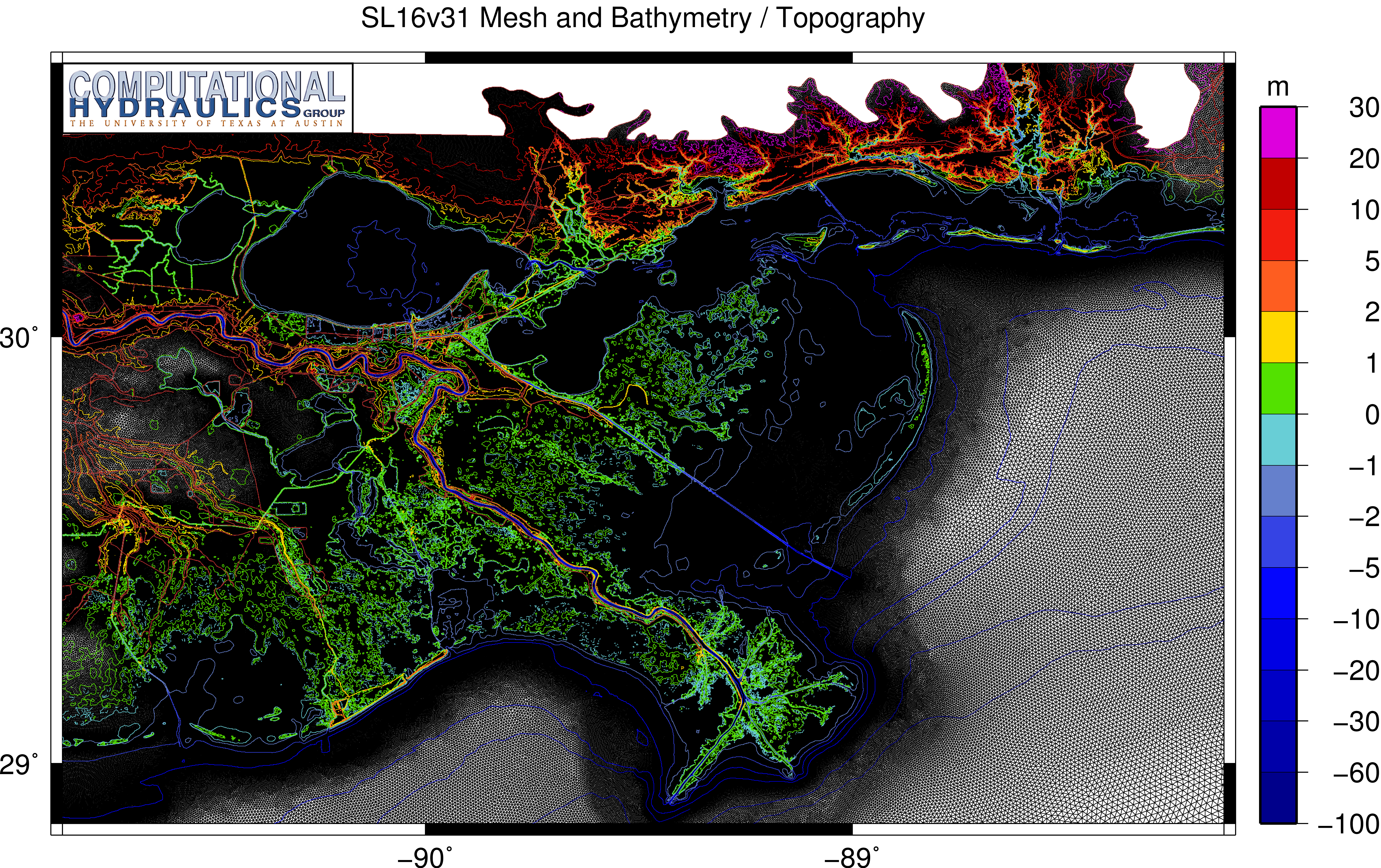
In this example, the mesh is again plotted, but now the triangular elements are shown in black, and the bathymetry/topography is shown with contour lines. This choice shows both the variability in the mesh resolution as well as the intricacy of the representation of the system. As the elements become smaller, the mesh is shown to transition from shades of gray to black. And, within the marshes and channels, the rapid changes in bathymetry are shown with tightness of the contour lines.
- FG49_04_Files
- FG49_04_SL16v31_Grid-Contours_SELA.inp
- TopoRainbow.pal
- TopoRainbow.txt
- CHG.eps
The contour lines require typically the most time for plotting by FigureGen. It can plot contour lines of mesh bathymetry, output quantities, etc., but these contour lines must be created dynamically by GMT. It is not possible to pass them to FigureGen in the same way as it reads the ADCIRC files. So it is recommended that the user start with relatively few contour lines and then add complexity if necessary.
5. Mesh decomposition with coastline schematic.
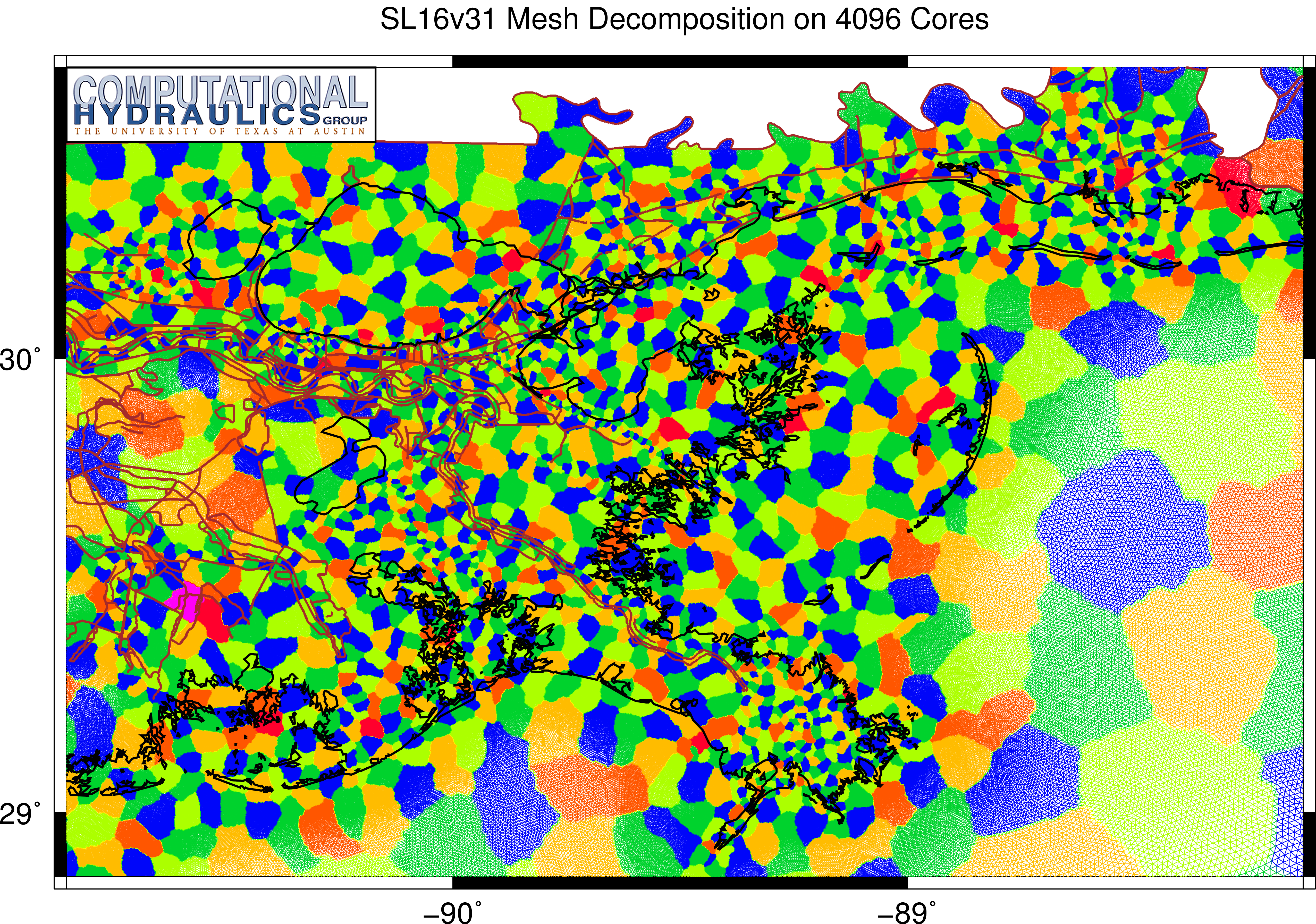
FigureGen can also plot the domain decomposition. As part of its pre-processing in a parallel computing environment, ADCIRC uses METIS to partition the input files. For example, a local mesh file is created for each core. The figure depicts how the SL16 mesh can be partitioned into 4096 local sub-meshes, each shown in a different color. Information is passed between cores at the boundaries of these local sub-meshes.
- FG49_05_Files
- FG49_05_SL16v31_Grid-Decomp_SELA.inp
- Decomp.pal
- CHG.eps
The plotting of the domain decomposition requires the use of the partmesh.txt file created by ADCIRC’s pre-processing program. Each line of this file corresponds to a mesh vertex, and the number on each line indicates the local sub-mesh on which the vertex resides. Using this information, FigureGen can reproduce the domain decomposition. The color scheme is optimized to require adjacent sub-meshes to be plotted in different colors.
As shown in this figure, the sub-meshes are created with a relatively constant number of elements and vertices, meaning that their spatial areas must decrease in regions with high levels of mesh resolution. In the offshore regions, the sub-meshes are larger, while in the floodplains, the sub-meshes are smaller. This variability becomes evident when a schematic of the coastline is added to the figure. Behind the barrier islands and onshore, the mesh resolution is increased, and thus the spatial areas of the sub-meshes decrease.
6. Nodal attribute of wind reduction factors with coastline schematic.
Besides the unstructured mesh, FigureGen can also plot the nodal attributes (from the fort.13 file). This example shows the wind reduction factors, which are used to decrease the forcing when the winds approach over rough terrain. ADCIRC searches upwind in 12 directions from each mesh vertex, and then uses the land usage types to determine how much the wind forcing should be reduced. Near open water, the full marine-strength winds are applied, and thus the wind reduction factors are near zero. But inland, especially in regions with tree cover, the winds can be reduced significantly.
- FG49_06_Files
- FG49_06_SL16v31_WindReduction_SELA.inp
- Default2.pal
- CHG.eps
This example plots the wind reduction factors for all 12 directions. If you want to plot only one direction, then the FigureGen input file would need to be changed so that the contour file format flag:
13-WIND-REDUCTION
is appended with a number between 1-12 to indicate the desired direction. For example, by setting the format to:
13-WIND-REDUCTION-4
the user would plot the wind reduction factors from the fourth direction, which corresponds to northward winds.
7. Nodal attribute of Manning’s n values with coastline schematic.
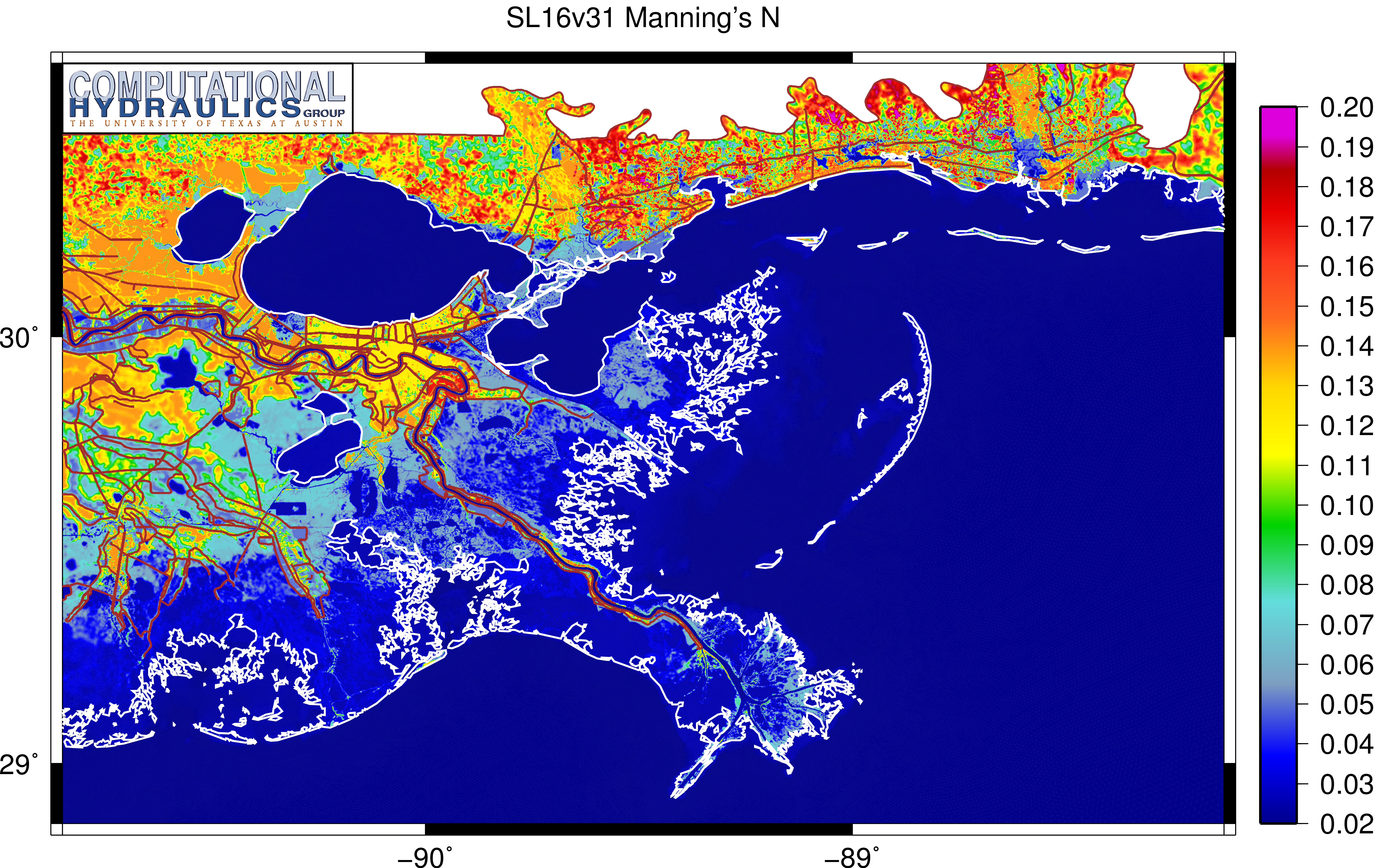
Another example of the plotting of nodal attributes is the Manning’s n values. These values are also assigned based on land usage types, using a spatial average onto each mesh vertex. Offshore, the Manning’s n values range downward to 0.012. In the marshes, the values are in the range of 0.05-0.06, and higher values exist inland.
- FG49_07_Files
- FG49_07_SL16v31_ManningsN_SELA.inp
- FG49_07_SL16v31_ManningsN_SELA_KMZ.inp
- Default2.pal
- CHG.eps
- CHG.png
We also include a schematic of the coastline, shown in white, to better delineate the higher Manning’s n values inland. The resulting image is a good representation of the spatial variability in the nodal attributes.
Another alternative:
 This plot can also be geo-referenced for use with software such as Google Earth. The image is prepared without borders, scales, plot labels, etc., and then everything is bundled into a KMZ file. This interaction with Google Earth is controlled with settings near the bottom of the FigureGen input file, where the user specifies the creation of the KMZ file and the desired lower layer of images. Click the image to download the KMZ file.
FigureGen will create a KMZ file that contains all of the images and other support files for use in Google Earth. The user can control the transparency and animations of the images as they are referenced to the world surface.
8. Contours and contour lines with labels and hurricane track.
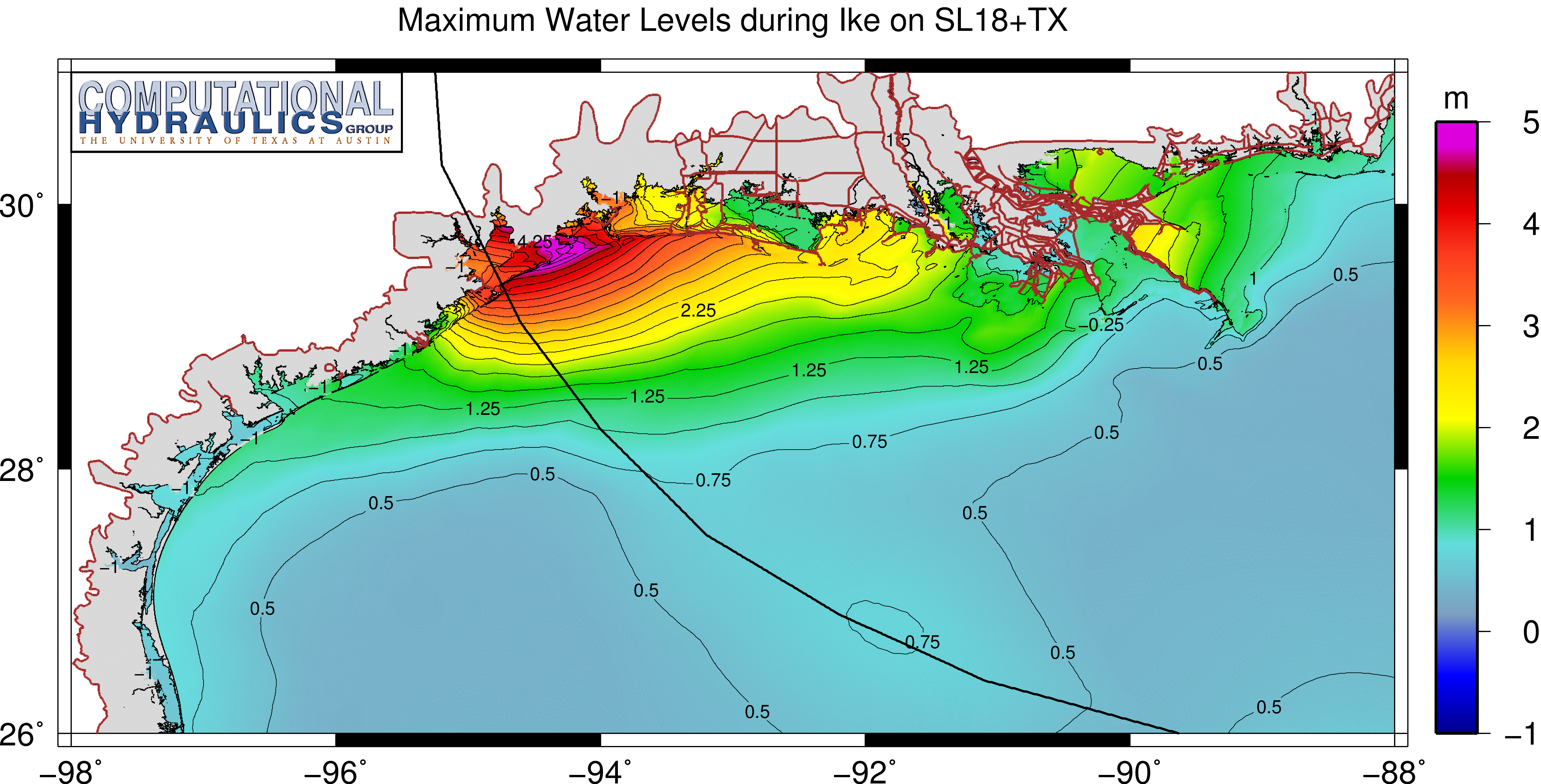
We can also plot the output from SWAN+ADCIRC. In this example, the maximum water levels (from the maxele.63 file) from Hurricane Ike are shown within Louisiana and Texas and on the continental shelf. We used the new SL18+TX mesh to generate these results; this mesh contains unprecedented levels of resolution along the entire coastlines of these two states, and thus it captures well the large-scale impact of Ike.
- FG49_08_Files
- FG49_08_SL18+TX_Ike_MaxEle_LATEX.inp
- FG49_08_SL18+TX_Ike_MaxEle_LATEX_GRF.inp
- Default2.pal
- IkeTrack.txt
- CHG.eps
The water levels are plotted both with colored contours and contour lines. These contour lines are also labeled using instructions from the FigureGen input file. We apply labels to every contour line, with the restriction that the labels must be at least 0.5in apart on the figure. The labels use a font size of 8pt, and they are not rotated. In addition to the labels, we also plot the storm track from an external text file.
Another alternative:
 This plot can also be geo-referenced for use with software such as ArcGIS. The image is prepared without borders, scales, plot labels, etc., and a world file is also created. This geo-referencing is controlled by a line near the end of the FigureGen input file. This line triggers the geo-referencing and sets the desired lower layer of images. Click the image to download a ZIP file.
In this example, FigureGen prepares the top-layer image in the same way as before, but we have disabled the lower layers to save time. These layers can be enabled by changing the line near the end of the FigureGen input file.
9. Contours and vectors with hurricane track.

Another example of the plotting of SWAN+ADCIRC output is this animation of the significant wave heights on the Louisiana-Texas continental shelf during Hurricane Ike. The storm intensified before it moved onto the shelf, and the significant wave heights increased to 15-16m to the northeast of the eye of the storm. These waves dissipated as they approached shallow water and the coastline.
- FG49_09_Files
- FG49_09_SL18+TX_Ike_HS-Wind_LATEX.inp
- FG49_09_SL18+TX_Ike_HS-Wind_LATEX_KMZ.inp
- Default2.pal
- IkeTrack.txt
- CHG.eps
- CHG.png
In this example, FigureGen generates images for all of the time snaps contained in the SWAN+ADCIRC output files. The user can specify the snaps for which to generate images, by listing them at the end of the FigureGen input file. It is also possible for FigureGen to generate images for all of the time snaps, by setting the number of snaps to zero.
Another alternative:
 This plot can also be geo-referenced for use with software such as Google Earth. The images are prepared without borders, scales, plot labels, etc., and then everything is bundled into a KMZ file. This interaction with Google Earth is controlled with settings near the bottom of the FigureGen input file, where the user specifies the creation of the KMZ file and the desired lower layer of images.
FigureGen will create a KMZ file that contains all of the images and other support files for use in Google Earth. The user can control the transparency and animations of the images as they are referenced to the world surface.
10. Contours of differences with hurricane track.
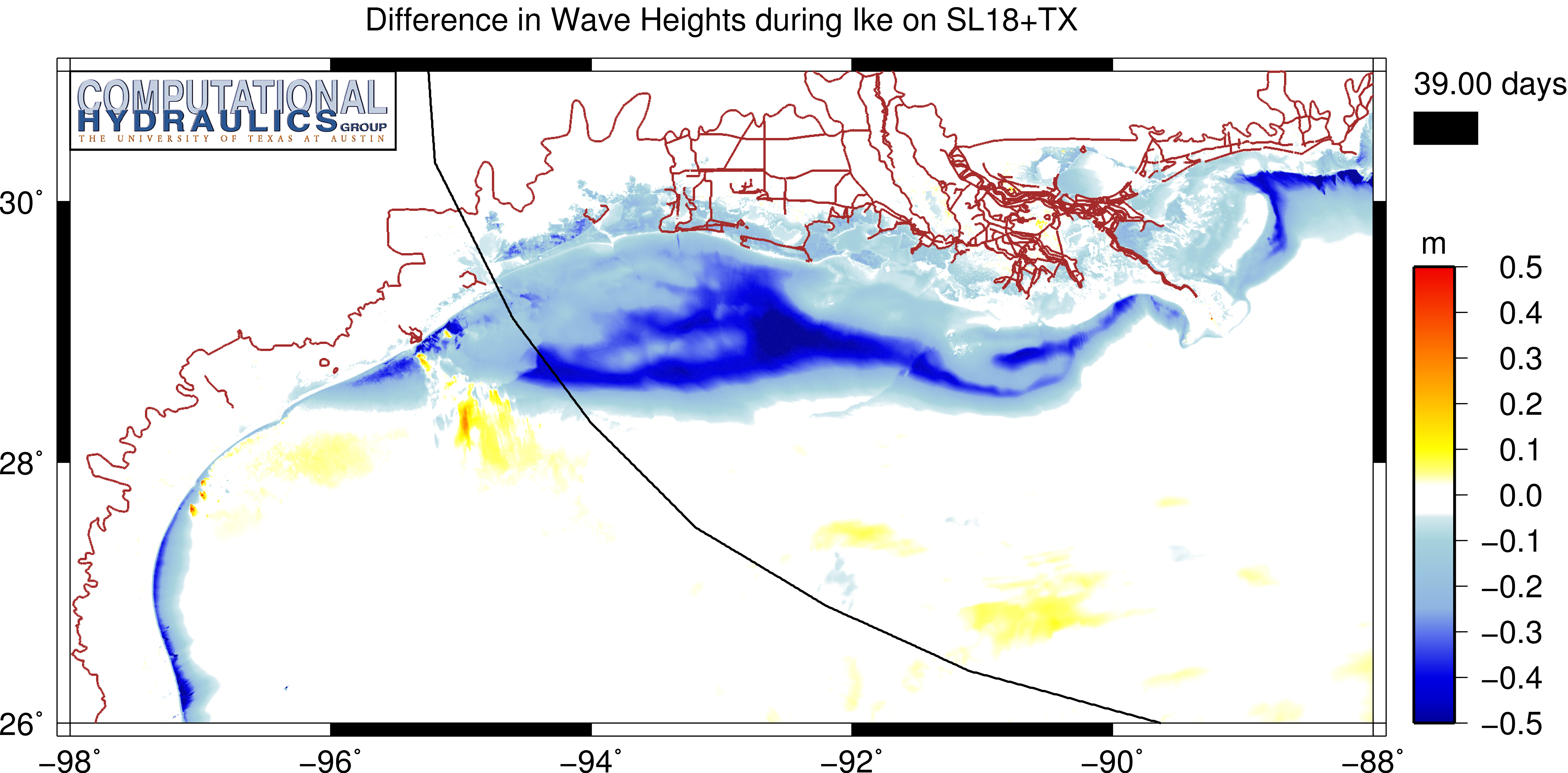
FigureGen can compute differences between input files and contour the results. In this example, we show the effect of the SWAN friction formulation on the maximum significant wave heights during Ike on the SL18+TX mesh. The difference is between: (a) results using our new formulation, which converts the Manning’s n values into roughness lengths for use by SWAN, and (b) the standard JONSWAP formulation with a constant coefficient of 0.038. The new formulation increases the friction on the continental shelf, and thus the significant wave heights are smaller, by as much as 0.5m.
- FG49_10_Files
- FG49_10_SL18+TX_Ike_MaxHSDiff_LATEX.inp
- GMT_CorpDiff.cpt
- IkeTrack.txt
- CHG.eps
The user does not need to pre-compute the differences before using FigureGen. Instead, the names of both SWAN+ADCIRC output files are specified in the FigureGen input file, and it computes internally the differences before plotting. Note that the difference is taken as the first results less the second results. Differences can be computed and plotted for output files, as shown here, but also for input values such as mesh bathymetry and other nodal attributes. The only restriction is that the mesh geometry must be the same.
Note also that this example employs a palette in a different format: CPT. By changing the palette format specification in the input file, FigureGen knows to work with this format.
11. HWM differences with background image.
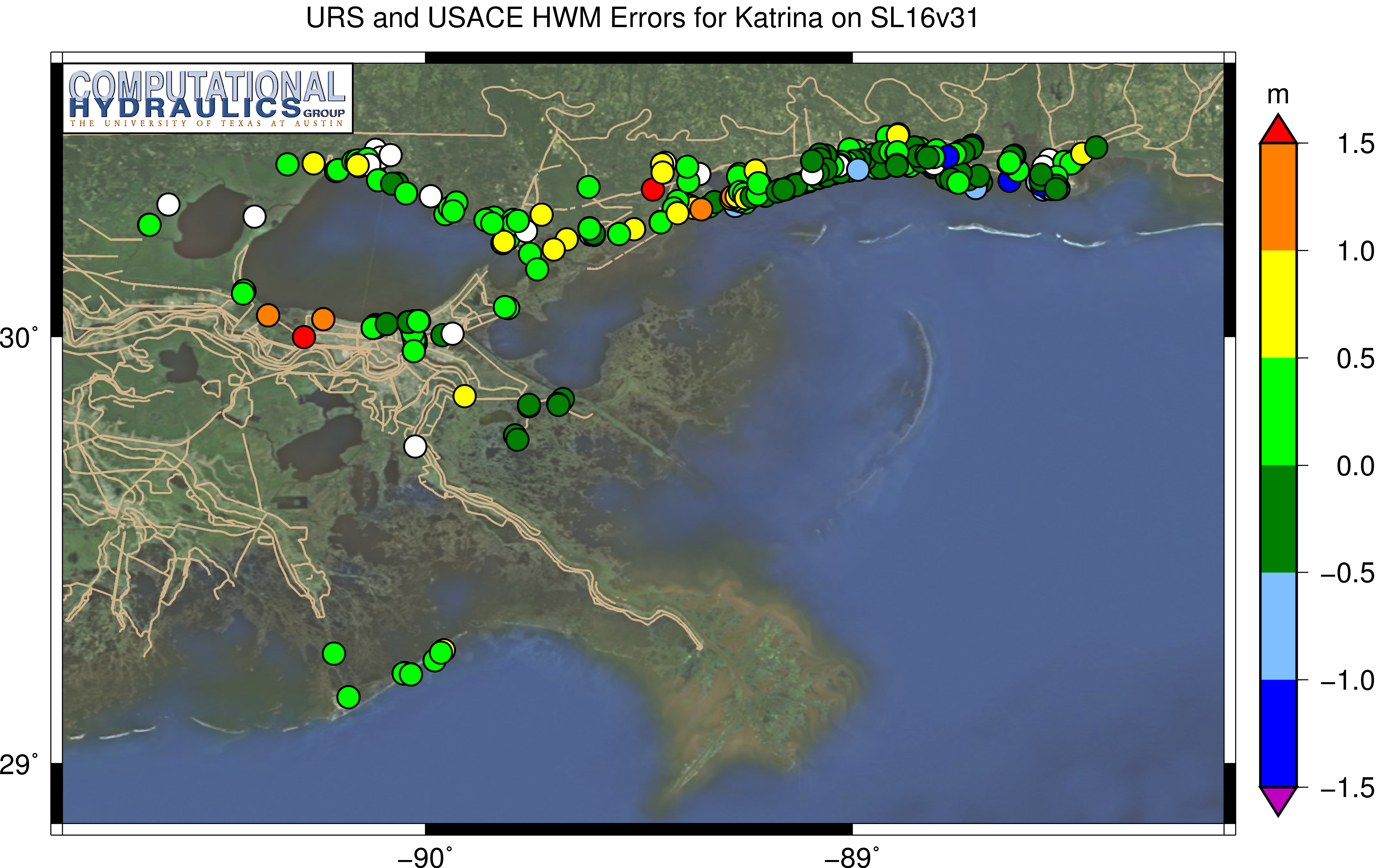
Besides contours and contour lines, FigureGen can also plot the differences at a set of high-water marks (HWMs) based on information in a comma-separated value (CSV) file. The result is a graphical representation of the magnitudes of the differences and where they are located. The example image shows the differences from our SWAN+ADCIRC hindcast of Katrina at the 399 HWMs collected by the USACE and the URS/FEMA in Louisiana, Mississippi and Alabama. The majority (80 percent) of these differences are within 0.5m.
- FG49_11_Files
- FG49_11_SL16v31_Katrina_HWM_SELA.inp
- HWM.cpt
- CHG.eps
- SatelliteImages.txt
- Satellite-SELA.png
- Satellite-SELA.pgw
These HWMs are specified as a CSV file with the following format:
lon,lat,bath,measured,modeled,error
but FigureGen reads only the first, second and sixth columns. We also make the following changes to the FigureGen input file: turn off the filled contours and contour lines, set the contour file format to HWM-CSV, specify a special HWM.cpt color palette, and set the number of times to split intervals at unity. This last setting will remove the smoothness in the color palette and establish clear bins for the different errors.
We also add a satellite image in the background. The background images are controlled via a separate text file. Each line in this file contains the time snap for which to apply the background image, the background image itself, and an associated world file for the geo-referencing. FigureGen will use the geo-referencing information to place the background image in the correct location relative to the user-defined longitude/latitude region in the FigureGen input file. Then it will add the rest of the contours, vectors, labels, etc. as layers above the background image.
Note that FigureGen requires the convert command from ImageMagick to process the background images. You will need to install ImageMagick and add the convert command to your environment variables.
12. Working with output files in NetCDF format.

In ADCIRC version 50, the NetCDF output format has been improved and expanded to include the output files containing SWAN values. Now the NetCDF-formatted output is a robust option in the model, and its use is increasingly widespread. NetCDF offers the obvious benefits of smaller file sizes and faster access. This new version of FigureGen is compatible with the NetCDF-formatted output files from SWAN+ADCIRC.
- FG49_12_Files
- FG49_12_SURA-UL_Ike_Ele-Wind_LATEX.inp
- Default2.pal
- IkeTrack.txt
- CHG.eps
In the example above, the water levels and wind velocities are plotted for a simulation of Ike on the SURA UltraLight mesh, which provides coverage of the northwestern Gulf and the adjacent floodplains. Ike was very large in size, and its winds caused flooding along the entire coastlines of Louisiana and Texas.
The NetCDF-formatted output files can be listed in the FigureGen input file in the same way as the ASCII-formatted output files. FigureGen must be compiled to include the NetCDF libraries (as described in the section above on ‘How to Compile’). But then it will detect automatically the format of the output file, and it will read it accordingly. The NetCDF files also contain information about the mesh itself, so they can be used in place of the ADCIRC mesh file. In this example, note that the mesh file is specified in the FigureGen input file to be the fort.63.nc file, and not the fort.14 file as usual.
Another alternative:
 You don’t have to use the NetCDF version of ADCIRC to benefit from this new NetCDF capability in FigureGen! It is recommended that you convert your output files from ASCII to NetCDF format before using them in FigureGen. This conversion will make it easier for FigureGen to read the files, and increase the speed at which it can produce the images.
The adcirc2netcdf program was written by Corbitt Kerr and is available as a utility from the ADCIRC Web site. This program will convert output files from ASCII to NetCDF format, including the writing of the mesh information to the NetCDF files. This conversion requires an investment of time, but it will pay off in faster FigureGen runs.
13. Lagrangian particles with water-level contours and wind vectors.
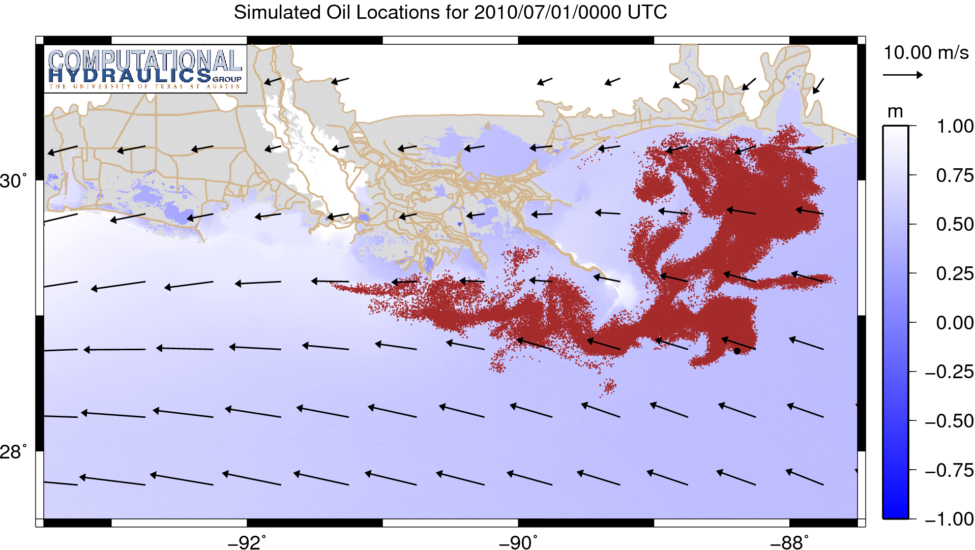
As part of our response to the spill following the destruction of the Deepwater Horizon drilling platform in 2010, we used a Lagrangian particle tracking model to predict the movement of the oil in the northern Gulf. The following image shows the predicted oil locations on 01 July 2010, or about two days into this forecast. During this time period, Hurricane Alex was moving through the southern Gulf, so the winds were easterly and relatively strong near Louisiana. The oil particles are being pushed into the marshes and along the coastline toward Texas.
- FG49_13_Files
- FG49_13_Particles_Ele-Wind_NGOM.inp
- FG49_13_Particles_Ele-Wind_NGOM_GRF.inp
- Blue.pal
- Stations.txt
- CHG.eps
The plotting of the particles is controlled by new lines in the middle of the FigureGen input file. The particle locations are specified in a file that can be in either ASCII or NetCDF format. In ASCII format, the file should look something like:
TextString

NumSnaps NumParticles TimeStep

for IS=1,NumSnaps

   RealTime NumParticles

   for IP=1,NumParticles

      ParticleNumber ParticleLon ParticleLat ParticleClass

   end IP loop

end IS loop
where the quantities in bold appear in the file. So the format is not too different from that of the ADCIRC global output files (fort.63, fort.74, etc.), in that the information is provided at each time snap and at every mesh vertex. In this case, for each time snap during the simulation, the longitude/latitude location is provided for each particle. There is also a column containing optional class information for the particles, but these classes are ignored by FigureGen.
In NetCDF format, the ncdump command should show something like:
dimensions:

   ntimesnap = UNLIMITED ; // (151 currently)

   nparticle = 10779434 ;

variables:

   double Time_index(ntimesnap) ;

   double X_particle(ntimesnap, nparticle) ;

   double Y_particle(ntimesnap, nparticle) ;

   double Z_particle(ntimesnap, nparticle) ;

}
where the X_particle and Y_particle variables contain the longitude/latitude locations of the particles. If FigureGen is compiled for use with NetCDF (as described above), then it will plot the particles from this file.
The other lines in the FigureGen input file control the plotting of the particles. For large data sets, the user can increase the speed of the plotting by using a subset of every N particles. (This example contains almost 11M particles, but FigureGen is set to plot every 100th particle.) The user can also control the size and color of the particles in the plot.
Another alternative:
 This plot can also be geo-referenced for use with software such as ArcGIS. The images are prepared without borders, scales, plot labels, etc., and a world file is also created. This geo-referencing is controlled by a line near the end of the FigureGen input file. This line triggers the geo-referencing and sets the desired lower layer of images. Click the image to download a ZIP file. In this example, FigureGen prepares the top-layer image in the same way as before, but it also prepares the images for the third layer, to maintain the desired resolution as the user zooms into specific regions of Louisiana.
14. Lagrangian particles with background images.
To validate our predictions of oil transport, we compared the locations of our Lagrangian particles with the observed oil slick extents from the available satellite imagery. The observations are shown in solid blue, while the predictions are shown in hatched red. At the beginning of the simulation, the observations and predictions are overlapped, but they diverge as time progresses.
- FG49_14_Files
- FG49_14_Particles_Satellite-Images_NGOM.inp
- FG49_14_Particles_Satellite-Images_NGOM_KMZ.inp
- DeepSkyBlue-Constant.pal
- Stations.txt
- CHG.eps
- CHG.png
- BackgroundImages.txt
- 20100629_0044.png
- 20100629_0044.pgw
FigureGen can plot this comparison through the use of background images. In the above animation, the observed slick extents are shown in navy blue at 10 time snaps as Hurricane Alex moved through the southern Gulf. These slick extents are supplied in separate images, which are then applied by FigureGen as the lower-most layer in the image. Everything else is plotted above the background images.
The background images are controlled via a separate text file. Each line in this file contains the time snap for which to apply the background image, the background image itself, and an associated world file for the geo-referencing. FigureGen will use the geo-referencing information to place the background image in the correct location relative to the user-defined longitude/latitude region in the FigureGen input file. Then it will add the rest of the contours, vectors, labels, etc. as layers above the background image.
Note that FigureGen requires the convert command from ImageMagick to process the background images. You will need to install ImageMagick and add the convert command to your environment variables.
Once the observed slick extents were in place, we did not want them to be obscured by the Lagrangian particles. In this example, the particles are shown with a pattern of red hatching, which gives an idea of the locations of the particles, but it also allows the observations to be seen. The pattern is specified in the FigureGen input file and corresponds to the numbering given in Appendix E of the GMT Documentation. The hatching in this example is pattern 7.
Another alternative:
 This plot can also be geo-referenced for use with software such as Google Earth. The images are prepared without borders, scales, plot labels, etc., and then everything is bundled into a KMZ file. This interaction with Google Earth is controlled with settings near the bottom of the FigureGen input file, where the user specifies the creation of the KMZ file and the desired lower layer of images. Click the image to download the KMZ file.
FigureGen will create a KMZ file that contains all of the images and other support files for use in Google Earth. The user can control the transparency and animations of the images as they are referenced to the world surface.